The problem
This one’s from Codeforces Round 1097 (Div. 1), problem B — Zhily and Barknights.
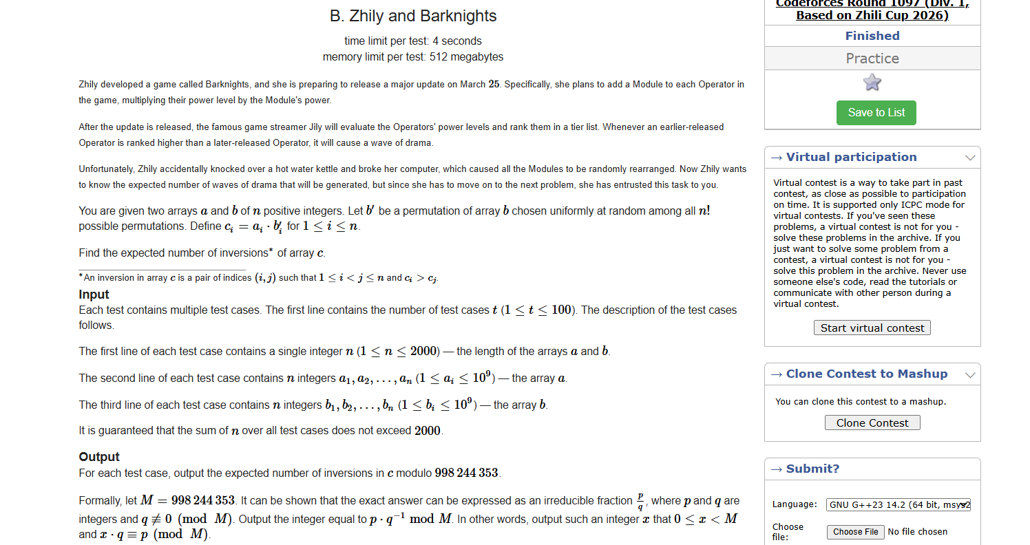
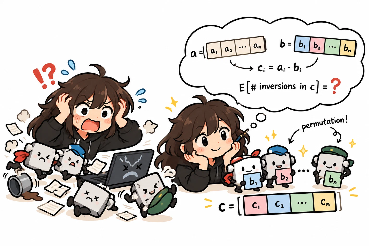
The gist: you’re given two arrays and of length . You take a uniformly random permutation of , define , and you need the expected number of inversions in , modulo . Constraints: , but across test cases, and .
The math for this problem was correct from my first submission. What was wrong was the data structure I used to implement it — that choice cost me two TLEs before I worked out exactly why, and by how much.
The idea (short version)
Expected inversions is a linearity-of-expectation problem. For a fixed pair of positions , you average over all ways to assign -values to them. Instead of thinking permutation-by-permutation, you can restructure the sum so that you sweep from left to right, and for each , you compare against every pair seen so far (all inserted incrementally) — using a Fenwick tree / order-statistics structure to count how many prior values are bigger or smaller in instead of per comparison.
Concretely, my final (accepted) solution keeps two structures:
prodTree— holds every product seen for indices processed so faraTree— holds every raw seen so far
and for each new , before inserting it, it queries: “how many things bigger than my current candidate are already in here?” That count feeds directly into the running inversion total.
I won’t paste the whole solve function in one block. I’ll go through it piece by piece further down, after covering the theory behind the data structure, since that’s what actually explains the TLE.
Attempt #1: PBDS ordered_multiset
My first working version used GNU’s Policy-Based Data Structures — specifically the tree container with tree_order_statistics_node_update, aka the thing every competitive programmer calls an “order statistics tree” or ordered_set / ordered_multiset.
typedef tree<
    pair<int, int>,
    null_type,
    less<pair<int, int>>,
    rb_tree_tag,
    tree_order_statistics_node_update>
ordered_multiset;
It compiled, gave the right answer on the sample cases, and I submitted it.
381028293   TLE on test 3   4000 ms   145200 KB
381028795   TLE on test 3   4000 ms   157200 KB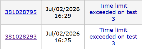
Two attempts, both failing on the same test. At that point I didn’t think much, later saw the math behind it.
To understand where the time was going, it helps to understand what ordered_multiset actually is under the hood. So let’s build up a Red-Black tree from the basics.
Part 1 — Why a plain BST isn’t enough
A Binary Search Tree is a tree where, for every node, everything in the left subtree is smaller and everything in the right subtree is bigger.
        5
      /   \
     3     8
    / \
   1   4
Search, insert, and delete all walk down from the root, so their cost is proportional to the height of the tree. If you’re lucky and the tree stays bushy, height is about , and everything is fast.
But if you insert values in sorted order — 1, 2, 3, 4, 5 — the tree degenerates into a straight line:
1
 \
  2
   \
    3
     \
      4
Now height equals , not , and every operation costs . This is the reason self-balancing trees exist: they force the height to stay logarithmic regardless of insertion order.
Part 2 — The Red-Black invariants
A Red-Black tree colors every node red or black and enforces five rules:
- Every node is red or black.
- The root is black.
- Every null leaf is treated as black.
- A red node never has a red child — no two reds in a row on any path.
- Every path from a node to any of its null descendants passes through the same number of black nodes (its “black-height”).
Rule 5 is the one doing the real work. It doesn’t force every path to be the same length — it forces the number of black nodes on every path to match. Combined with rule 4 (reds can’t stack), this caps how much longer any path can be than any other: at most a factor of 2.
The proof that height stays
Define as the black-height of node : the number of black nodes from down to a null leaf (not counting itself).
Lemma. A subtree rooted at contains at least internal nodes.
Proof, by induction on subtree height.
Base case: is a null leaf. , subtree contains nodes. True.
Inductive step: each child of has black-height either (if the child is red) or (if the child is black). Either way, by the inductive hypothesis each child’s subtree has at least nodes, so:
Now, because rule 4 forbids two reds in a row, at least half the nodes on any root-to-leaf path are black, so if is the tree’s height:
Plugging into the Lemma with = total nodes:
That’s the guarantee. However you insert data, height never exceeds roughly twice .
Part 3 — Fixing violations: rotations
When you insert a new node, it always starts red (inserting black would instantly break rule 5 on one path; inserting red might break rule 4, which is locally repairable).
If the new node’s parent is black, nothing broke — done. If the parent is also red, you have two reds in a row, and you fix it based on the color of the “uncle” (the parent’s sibling):
Case A — uncle is red. Just recolor: parent → black, uncle → black, grandparent → red. Then recheck one level higher, since the grandparent turning red might itself clash with its parent.
Case B — uncle is black or missing. You need a rotation. A left rotation around node with right child : takes ’s spot, becomes ’s left child, and ’s old left subtree becomes ’s new right subtree.
   P                R
    \              / \
     R     -->    P   (R's old right)
    / \             \
  (R's  (R's old      (R's old left)
  old   right)
  left)
It’s three pointer reassignments — work — but it locally reshuffles the shape of the tree. A right rotation is the mirror image. Depending on whether the violation is a “straight line” or a “zig-zag,” you need one rotation plus a recolor, or two rotations plus a recolor.
A worked example
Insert 10, 20, 30, 15, 5 one at a time.
Insert 10 — tree is empty, becomes root, forced black.
10(B)Insert 20 — goes right of 10, colored red. Parent is black, no violation.
10(B)
    \
    20(R)
Insert 30 — goes right of 20, red. Now 20(R) has red child 30(R) — violation. Uncle is nil (black), straight-line case → rotate left at 10.
      20(B)
     /    \
  10(R)  30(R)
Insert 15 — 15 < 20, go left to 10; 15 > 10, becomes 10’s right child, red.
        20(B)
       /    \
   10(R)   30(R)
       \
      15(R)
10(R) has red child 15(R) — violation. Uncle (30) is red → Case A: recolor 10 and 30 to black, 20 to red, then re-check from 20. Since 20 is root, force it back to black.
        20(B)
       /    \
   10(B)   30(B)
       \
      15(R)
Insert 5 — 5 < 20 → left to 10; 5 < 10 → becomes 10’s left child, red. Parent (10) is black, no violation.
        20(B)
       /    \
   10(B)   30(B)
   /    \
 5(R)  15(R)
Tree is balanced, all 5 rules hold.
Part 4 — Turning it into an order-statistics tree
A plain std::set is a Red-Black tree, but it can’t answer “how many elements are smaller than ?” or “what’s the -th smallest element?” in — because a node in a plain RB tree only knows its own key and its children’s pointers. It has no idea how many descendants it has.
tree_order_statistics_node_update fixes this by attaching one extra integer to every node: subtree_size.
int sizeOf(Node* n) { return n ? n->size : 0; }

void updateSize(Node* n) {
    if (n) n->size = 1 + sizeOf(n->left) + sizeOf(n->right);
}
Every insert, delete, or rotation calls this update on the handful of nodes it touched. Since a rotation only changes the parent/child relationship of two nodes ( and ), only their sizes need recomputing — and in a specific order:
void rotateLeft(Node* x) {
    Node* y = x->right;
    x->right = y->left;
    if (y->left) y->left->parent = x;
    y->left = x;
    // ... parent pointer bookkeeping omitted for brevity ...
    updateSize(x);   // x's children changed -> fix x first
    updateSize(y);   // y's size depends on x's corrected size
}
Why nothing above needs updating: a rotation doesn’t add or remove any nodes from the tree — it just reshuffles which nodes are whose children. Every node outside still has exactly the same descendants it had before. Since size is purely a function of a node’s current children, only and can possibly have a new size, and must be recomputed after because ’s children now include the corrected .
The two payoff operations
order_of_key(q) — count of elements strictly less than :
int order_of_key(int q) {
    Node* x = root;
    int count = 0;
    while (x) {
        if (q > x->key) {
            count += sizeOf(x->left) + 1;
            x = x->right;
        } else {
            x = x->left;
        }
    }
    return count;
}
Correctness, by induction on the walk. If , then every node in ’s left subtree is (that’s matches), and itself is also (+1 more) — so we add exactly and recurse right, where any remaining smaller-than- elements must live. If , then and its whole right subtree are , contributing nothing, and we recurse left. Both branches preserve the invariant “count so far is exactly correct for everything already visited,” so by induction the final count is exact.
find_by_order(k) — the -th smallest element:
Node* find_by_order(int k) {
    Node* x = root;
    while (x) {
        int L = sizeOf(x->left);
        if (k < L) x = x->left;
        else if (k == L) return x;
        else { k -= (L + 1); x = x->right; }
    }
    return nullptr;
}
Both run in time proportional to the height of the tree, which we already proved is . So on paper, this gives a fully indexable, rank-queryable balanced BST at per operation.
check it’s uses here.
Part 5 — Counting exactly how many operations my code did
Here’s the structure of the hot loop in my first (TLE’d) solution:
rep(i, 0, n) {
    rep(j, 0, n) {
        int g = prodTree.order_of_key({a[i]*b[j], INF});
        int h = aTree.order_of_key({a[i], INF});
        // ... accumulate into total ...
    }
    rep(j, 0, n) {
        prodTree.insert({a[i]*b[j], prodTimer++});
    }
    aTree.insert({a[i], aTimer++});
}
Let’s count every single operation exactly, for (the worst case, since still allows one test case with ).
| Operation | How many times | Which tree | Max size that tree reaches |
|---|---|---|---|
order_of_key on prodTree | prodTree | ||
order_of_key on aTree | aTree | ||
insert into prodTree | prodTree | ||
insert into aTree | aTree |
Total tree operations:
For , :
Twelve million operations isn’t a large number on its own — modern CPUs execute billions of instructions per second. The important question is what each of these operations actually costs on real hardware, not just in theory.
Cost per operation, using the height bound we proved
prodTree grows up to entries:
aTree grows up to entries:
Total pointer traversal steps across the whole run:
Turning pointer hops into wall-clock seconds
This is where the TLE actually comes from. A pointer hop in a tree made of heap-allocated nodes isn’t free the way an array index is. Every node was allocated separately by new, so nodes end up scattered across essentially random addresses in RAM. Walking parent → child → child means jumping between memory locations the CPU has no way to predict in advance.
Modern CPUs read memory in 64-byte cache lines and keep recently-used lines in small, extremely fast caches (L1, L2, L3). Rough costs on a typical 3 GHz machine:
- L1 cache hit: ~4 cycles ≈ 1 ns
- Main memory (cache miss): ~300 cycles ≈ 100 ns
Because each pointer hop in our 4-million-node tree lands on an essentially random address, almost every hop is a cache miss. Using the pessimistic-but-realistic 100 ns/hop figure:
On top of that, every insert calls new under the hood — heap allocations, at roughly 20 ns each once you include allocator bookkeeping and rebalancing overhead:
— negligible compared to the 44 seconds above, but not zero.
Estimated total: ~44 seconds. The actual time limit is 4 seconds — roughly 11x over budget, which matches what happened on both submissions: the judge simply hit the 4000ms cutoff.
In practice not every single hop costs the full 100 ns — the top few levels of an actively-used tree tend to stay in L2/L3 cache, which is why the real run finished in some large but finite time rather than a literal 44 seconds before Codeforces terminated it. But the order of magnitude, tens of seconds needed versus 4 allowed, is enough to explain the failure on its own.
The algorithmic complexity, , was completely correct. The problem was that the constant hidden inside that was roughly 100x larger than it needed to be, purely because of how the data was laid out in memory.
Attempt #2: swap the tree for a flat array
The fix keeps the exact same math — same comparisons, same accumulation logic — and only changes the data structure. Instead of a Red-Black tree of heap nodes, I use coordinate compression plus a Fenwick tree (Binary Indexed Tree) backed by one contiguous vector<int>.
First, compress every value I’ll ever query into a small rank:
vi vals;
rep(i, 0, n) {
    vals.pb(a[i]);
    rep(j, 0, n) vals.pb(a[i] * b[j]);
}
uni(vals); // sort + unique
A tiny helper turns any real value into its compressed rank via binary search:
auto get_id = [&](int x) {
    return lower_bound(all(vals), x) - vals.begin() + 1;
};
The Fenwick tree implementation is simple — just an array and two loops:
struct Fenwick {
    int n;
    vector<int> tree;
    Fenwick(int n) : n(n), tree(n + 1, 0) {}

    void add(int i, int delta) {
        for (; i <= n; i += lsb(i)) tree[i] += delta;
    }
    int query(int i) {
        int sum = 0;
        for (; i > 0; i -= lsb(i)) sum += tree[i];
        return sum;
    }
};
And the hot loop barely changes shape at all — order_of_key becomes query, insert becomes add:
rep(i, 0, n) {
    rep(j, 0, n) {
        int g   = prodTree.query(get_id(a[i] * b[j]));
        int hii = sz_prod - g;

        int h      = aTree.query(get_id(a[i]));
        int hiiiuu = sz_a - h;

        int diff = (hii - hiiiuu) % MOD;
        if (diff < 0) diff += MOD;
        total = (total + (diff * fact[n-2]) % MOD) % MOD;
    }
    rep(j, 0, n) {
        prodTree.add(get_id(a[i] * b[j]), 1);
        sz_prod++;
    }
    aTree.add(get_id(a[i]), 1);
    sz_a++;
}
(I also fixed a subtle negative-modulo bug along the way — diff can go negative before the % MOD, so it needs an explicit if (diff < 0) diff += MOD guard, and I precompute factorials once instead of recomputing an inverse in the inner loop.)
This submission passed:
381029218 Accepted 3625 ms 92900 KB
3625 ms, inside the 4000 ms limit. The algorithmic complexity didn’t change from the first attempt, so the difference has to come from somewhere else.
Part 6 — Why the Fenwick tree passes: same math, different constant
The Fenwick tree does the same number of “logical steps” as the PBDS tree — for , tree height was for the big structure and for the small one, and a Fenwick tree over the same number of elements needs the same iterations per add/query, since each step strips off the lowest set bit. The total operation count million and total “step” count are essentially identical to before.
The difference is entirely in what each step costs, physically.
A Fenwick tree is backed by one vector<int> allocated once, up front, as a single contiguous block of memory. Walking it means computing i -= lsb(i) or i += lsb(i) and jumping to a new array index — and because the whole array is one block, those jumps land inside memory the CPU has already loaded into cache, or can predict and prefetch, rather than jumping to a brand-new random heap address every single time.
For , the compressed value array vals has at most entries, so each Fenwick tree (prodTree, aTree) is a vector<int> of a few million 4-byte integers — a few tens of megabytes. That’s too big to fit entirely in L1 (usually 32–48 KB) or L2 (a few hundred KB to a few MB) cache, but:
- it fits comfortably in L3 cache on most modern CPUs (typically 8–32 MB), and
- even where it spills into RAM, sequential/strided access to one contiguous array is exactly the pattern hardware prefetchers are built to detect and pre-load ahead of time.
Redoing the same wall-clock estimate as before, but now assuming most accesses hit cache (say, an average of ~2 ns per step instead of ~100 ns, blending a mix of L1/L2/L3 hits with the occasional real RAM miss):
That’s roughly 50x faster than the ~44 second PBDS estimate, for the same number of logical steps. It also removes the other overhead the tree had: no new call on every insert (the vector for each Fenwick tree is allocated exactly once, up front), no red-black rebalancing, no rotations, no recoloring, no extra size bookkeeping through parent pointers.
The actual submission ran in 3625 ms rather than my rough 0.88s estimate — real code always carries extra constant factor from the modular arithmetic, the lower_bound binary searches for coordinate compression, and I/O — but it lands in the same universe as the estimate, and critically, on the correct side of the 4-second wall, instead of ~10x over it.
Summary
Both solutions are . Both perform roughly the same number of logical tree steps. The difference between the TLE and the accepted run came down to where the data physically lives in memory:
- A tree of individually
new’d nodes is scattered across RAM, so each traversal involves multiple unpredictable cache misses, each costing on the order of 100 ns. - A flat array backing a Fenwick tree is one contiguous block, so traversal is mostly cache hits and prefetch-friendly access patterns, each costing on the order of 1–2 ns.
Same time complexity, but a 50–100x difference in the constant factor, entirely due to memory layout. ordered_set and ordered_multiset are useful — for smaller operation counts they’re simpler to write and fast enough. But once the operation count reaches into the millions in a tight loop, that per-operation constant becomes the deciding factor, and a flat array-based structure like a Fenwick tree or segment tree is usually the better choice.
Here’s the minimal Fenwick tree itself, runnable and editable below. It reads n values followed by q inclusive [l, r] range-sum queries (0-indexed) and prints the sum for each — try changing the array or queries and hit Run, or use the test cases underneath to check it against a couple of known answers.
#include <bits/stdc++.h>
using namespace std;

struct Fenwick {
    int n;
    vector<long long> tree;
    Fenwick(int n) : n(n), tree(n + 1, 0) {}

    void add(int i, long long delta) {
        for (++i; i <= n; i += i & (-i)) tree[i] += delta;
    }
    long long prefixSum(int i) {
        long long sum = 0;
        for (++i; i > 0; i -= i & (-i)) sum += tree[i];
        return sum;
    }
};

int main() {
    int n;
    cin >> n;
    Fenwick fen(n);
    for (int i = 0; i < n; i++) {
        long long x; cin >> x;
        fen.add(i, x);
    }

    int q;
    cin >> q;
    while (q--) {
        int l, r; cin >> l >> r;
        long long sum = fen.prefixSum(r) - (l ? fen.prefixSum(l - 1) : 0);
        cout << sum << "\n";
    }
}ascending array, two ranges Input: Expected: includes a negative value Input: Expected:Test cases
5
1 2 3 4 5
2
0 2
1 46
143
10 -5 7
1
0 212